This article walks through the complete development of an interactive UFO sightings dashboard — from raw data sourcing and preprocessing, through geocoding 200,000 records, to a production React application with maps, charts, and filters. The app is live at parallel-perspectives.com/infographics/ufo-sightings-dashboard/.
1. Project Overview
The goal was to build an explorable, data-driven interface around NUFORC (National UFO Reporting Center) sighting reports spanning 1905 to 2023 — 147,890 records in total. The dashboard needed to support:
- A filterable world map with marker clustering
- Year, shape and country filters with URL-persisted state
- KPI cards and a full chart section
- A searchable event table with map focus
- A CSV export feature
- Dark mode support throughout
The tech stack: React, Webpack, Leaflet + leaflet.markercluster, Recharts, Tailwind CSS, and a Python preprocessing pipeline.
2. Data Sourcing and Format Decision
The original dataset was a CSV file from Kaggle, limited to sightings up to 2015. To extend coverage to 2023, I sourced the updated NUFORC dataset from Hugging Face, which provides the data as both CSV and JSON.
Why JSON over CSV
The original CSV was loaded client-side using d3.dsv(), which was noticeably slow in production — parsing a large delimited file in the browser main thread blocks rendering. Switching to JSON allows the browser to use its native JSON parser, which is significantly faster. More importantly, it enabled aggressive field pruning at the preprocessing stage.
The raw NUFORC JSON schema per record:
{
  "Sighting": 114864,
  "Occurred": "2014-09-21 13:00:00 Local",
  "Location": "Huntsville, TX, USA",
  "Shape": "Rectangle",
  "Duration": "several seconds",
  "No of observers": 1,
  "Reported": "2014-10-23 11:11:17 Pacific",
  "Posted": "2014-11-06 00:00:00",
  "Characteristics": ["Lights on object", "Aura or haze around object"],
  "Summary": "Rectangle shaped UFO observed traveling at an extremely high rate of speed.",
  "Text": "I observed a rectangle shaped UFO moving at a very high rate of speed..."
}
Fields dropped: Text (full witness narrative, accounts for ~60% of file weight), Posted, Reported. The Summary one-liner is sufficient for popup content. This brought the file from ~200MB down to ~49MB — still large, but manageable for a static asset served over HTTP.
Output schema
{
  "id": 114864,
  "date": "2014-09-21",
  "location": "Huntsville, TX, USA",
  "shape": "Rectangle",
  "duration": "several seconds",
  "observers": 1,
  "characteristics": ["Lights on object", "Aura or haze around object"],
  "summary": "Rectangle shaped UFO observed...",
  "lat": 30.7235,
  "lon": -95.5507
}
3. The Geocoding Pipeline
The raw dataset contains no coordinates — only freeform location strings. Since the map is the core feature of the dashboard, geocoding was a prerequisite.
Strategy: deduplicate before geocoding
With ~147,000 records but only ~7,000 unique location strings, geocoding row by row would be both wasteful and time-prohibitive. The pipeline instead:
- Extracts all unique location strings
- Geocodes only those unique values (via Nominatim)
- Joins coordinates back to all records
This reduced the number of API calls from ~147,000 to ~7,000 — a 95% reduction.
Location string cleaning
NUFORC location strings are inconsistently formatted. Several patterns required normalization before hitting the geocoder:
"Huntsville, TX, USA"                         → clean, no change needed
"Wollongong (Australia), , Australia"          → "Wollongong, Australia"
"Soulatge (near St. Paul) (France), , France" → "Soulatge, France"
"Kiev (Ukraine), , Ukraine"                   → "Kiev, Ukraine"
The cleaning logic strips all parenthetical groups with a single regex, then collapses consecutive empty comma-separated segments:
def clean_location(raw: str) -> str:
    s = re.sub(r'\([^)]*\)', '', raw)       # remove (parentheticals)
    s = re.sub(r'(\s*,\s*){2,}', ', ', s)  # collapse ,, into ,
    return s.strip(' ,')
Nominatim geocoding with resumable cache
Nominatim (OpenStreetMap) was chosen as the geocoder — free, no API key required, and handles international locations well. Its ToS requires a maximum of 1 request/second, which the pipeline respects with a configurable delay (default: 1.1s).
To handle interruptions gracefully, results are written to a local JSON cache every 50 requests. Rerunning the script skips already-cached locations. At ~7,000 unique locations and 1.1s per request, the full run takes approximately 2 hours.
def geocode(location: str, delay: float = 1.1) -> dict | None:
    params = {"q": location, "format": "json", "limit": 1}
    resp = requests.get(NOMINATIM_URL, params=params, headers=HEADERS, timeout=10)
    results = resp.json()
    time.sleep(delay)
    return {"lat": float(results[0]["lat"]), "lon": float(results[0]["lon"])} if results else None
Geocoding success rate was approximately 90–92%. Records with failed geocoding are retained in the output with null coordinates and filtered out of the map layer only — they still appear in charts and the table.
4. React Application Architecture
Data loading and normalization
Data is loaded via fetch() on mount, parsed, and split into two parallel arrays: data (all records, used for charts and filters) and mapData (records with valid coordinates only, used for the map):
useEffect(() => {
  fetch('data/nuforc_clean.json')
    .then(res => res.json())
    .then(raw => {
      const parsed = raw
        .map(d => ({
          ...d,
          year: d.date ? Number(d.date.split('-')[0]) : NaN,
          lat: d.lat ?? NaN,
          lon: d.lon ?? NaN,
          country: parseCountry(d.location),
        }))
        .filter(d => !isNaN(d.year));

      setData(parsed);
      setMapData(parsed.filter(d => !isNaN(d.lat) && !isNaN(d.lon)));
      setLoading(false);
    });
}, []);
The country field is derived at load time by extracting the last non-empty segment of the location string:
const parseCountry = (location = '') =>
  location.split(',').map(s => s.trim()).filter(Boolean).pop() || 'Unknown';
Filter state and URL persistence
Three filters are active simultaneously: year, shape, and country. Their state is persisted to the URL via URLSearchParams, enabling shareable links:
useEffect(() => {
  const params = new URLSearchParams();
  params.set('year', year);
  if (shape !== 'all') params.set('shape', shape);
  if (country !== 'all') params.set('country', country);
  window.history.replaceState({}, '', `?${params.toString()}`);
}, [year, shape, country]);
On initial load, URL params are read back to restore the previous state. If no year param is found, a random year is selected from years with more than 50 sightings — giving new visitors a populated map immediately.
Cascading filter options
Shape and country dropdowns are dynamically constrained to valid combinations given the current selection. This prevents users from ending up with empty results:
const shapes = useMemo(() => [
  'all',
  ...new Set(
    data
      .filter(d => d.year === year && (country === 'all' || d.country === country))
      .map(d => d.shape)
      .filter(Boolean)
  )
], [data, year, country]);
A separate useEffect resets filters that become invalid when the year changes — for example, if a shape existed in 2012 but not in 2015.
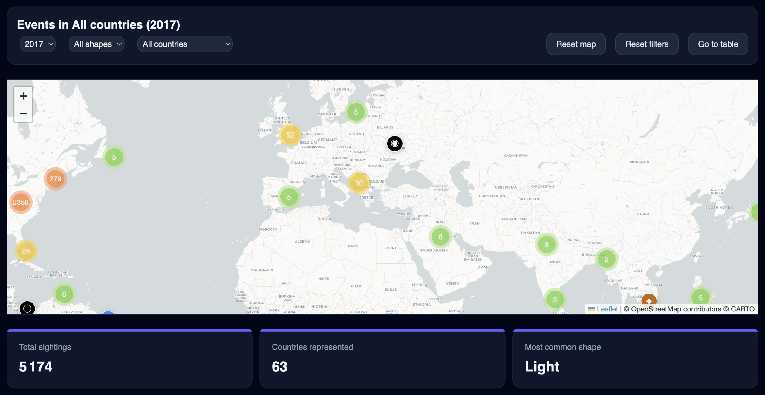
5. Map Implementation
The map uses Leaflet with leaflet.markercluster for performance at scale. Custom divIcon markers encode the sighting shape visually using symbols and colors:
const shapeIcons = {
  circle:    { symbol: '●', color: '#1E90FF' },
  triangle:  { symbol: '▲', color: '#4682B4' },
  light:     { symbol: '✦', color: '#BF6900' },
  fireball:  { symbol: '🔥', color: '#4169E1' },
  // ...
};
Clustering is disabled at zoom level 8 and above (disableClusteringAtZoom: 8), allowing individual markers to become visible when the user zooms into a region.
Map–table interaction
Selecting a row in the event table triggers a map pan and zoom to the corresponding marker, and opens its popup automatically:
onSelectLocation={d => {
  setCenter([d.lat, d.lon]);
  setZoom(8);
  setFocusEvent(d.id ?? `${d.date}-${d.location}`);
  setTimeout(() => mapSectionRef.current?.scrollIntoView({ behavior: 'smooth' }), 100);
}}
The focusEvent ID is matched against markers during the map render cycle, and marker.openPopup() is called with a 150ms delay to allow the map pan animation to complete first.
6. Dashboard Service Layer
All data aggregation is isolated in a dashboardService.js module, keeping components purely presentational. Each function takes the filtered dataset as input and returns a chart-ready array.
Key functions
getSightingsByMonth — extracts month from the ISO date string:
const month = parseInt(item.date.split('-')[1], 10) - 1;
getAverageDuration — parses free-text duration strings (“several minutes”, “2 hours 30 seconds”) using regex:
const hours   = raw.match(/(\d+\.?\d*)\s*hour/);
const minutes = raw.match(/(\d+\.?\d*)\s*min/);
const seconds = raw.match(/(\d+\.?\d*)\s*sec/);
getShapeEvolution — groups the top N shapes by decade, returning a stacked area chart-ready structure:
const decade = Math.floor(item.year / 10) * 10;
decades[decade][shape]++;
getCharacteristicsFrequency — flattens the nested characteristics arrays across all records:
item.characteristics.forEach(c => {
  counts[c] = (counts[c] || 0) + 1;
});
getTopCountries — derives country from location string rather than a dedicated field:
const country = (item.location || '')
  .split(',').map(s => s.trim()).filter(Boolean).pop() || 'unknown';
7. Chart Section
Eight charts are rendered using Recharts, laid out in a responsive two-column grid (xl:grid-cols-2):
| Chart | Type | Data source |
|---|---|---|
| Sightings over time | Line | Full dataset, all years |
| Top shapes | Horizontal bar | Filtered dataset |
| Top countries | Horizontal bar | Filtered dataset |
| Sightings by hour | Vertical bar | Filtered dataset |
| Sightings by month | Vertical bar | Filtered dataset |
| Most reported characteristics | Horizontal bar | Filtered dataset |
| Number of observers | Vertical bar | Filtered dataset |
| Shape evolution by decade | Stacked area | Full dataset, from 1950 |
The shape evolution chart spans the full width (xl:col-span-2) and uses a fixed color palette mapped to each shape series. It deliberately starts at 1950 — earlier data is too sparse to be meaningful.
Country and shape charts use dynamic heights based on the number of entries (length * 36 + 40), preventing label truncation regardless of how many items are present.
8. Loading State
Loading the 49MB JSON file takes a few seconds on a standard connection. A dedicated loading screen prevents a blank white flash:
if (loading) {
  return (
    <div className="flex min-h-screen flex-col items-center justify-center gap-6 bg-slate-950">
      <span className="text-5xl animate-pulse">🛸</span>
      <h1 className="text-2xl font-semibold text-slate-100">UFO Sightings Dashboard</h1>
      <p className="text-sm text-slate-400">Loading sighting data…</p>
      <div className="h-1 w-64 overflow-hidden rounded-full bg-slate-800">
        <div className="h-full w-full animate-[loading_1.5s_ease-in-out_infinite] rounded-full bg-slate-400" />
      </div>
    </div>
  );
}
The animated progress bar uses a custom Tailwind keyframe (translateX -100% → 100%) defined in tailwind.config.js.
9. Production Build
The app is bundled with Webpack 5. The main challenge was ensuring static assets (nuforc_clean.json, countries.geojson) were correctly copied to the dist/ folder and served at the expected paths. This is handled by copy-webpack-plugin:
new CopyPlugin({
  patterns: [{ from: 'public', to: '.' }]
})
The publicPath in the Webpack output config is set to a relative path rather than / to ensure the bundle works when hosted in a subfolder:
output: {
  filename: 'bundle.js',
  path: path.resolve(__dirname, 'dist'),
  publicPath: 'auto',
  clean: true,
}
10. Key Takeaways
A few decisions that proved particularly important over the course of the build:
Deduplicate before geocoding. Geocoding 7,000 unique locations instead of 147,000 rows saved roughly 38 hours of API time. The join back to the full dataset is trivial by comparison.
Separate map data from chart data at load time. Maintaining two arrays — one with all records, one with valid coordinates only — avoids repeated filtering on every render and keeps the map layer clean without sacrificing chart completeness.
Derive fields at load time, not at render time. Computing year and country once during the initial parse, rather than inside useMemo hooks, keeps the service functions simple and avoids redundant string operations on every filter change.
Keep the service layer pure. All aggregation functions take raw arrays and return plain objects. No component state, no side effects. This makes them trivially testable and easy to extend with new chart types.
The full source is not currently public, but feel free to reach out via parallel-perspectives.com if you have questions about any part of the implementation.